It is not uncommon to encounter errors in spreadsheets. But thankfully Microsoft has equipped Excel with tools to help resolve errors in Excel formula. This includes the ability to evaluate formula and set error checking options.
In this article we will cover step by step the options available to help resolve errors in Excel formula.
Tracing Formula Precedents and Dependents
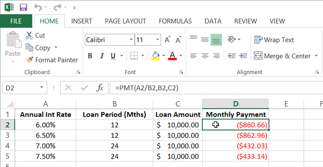
Tracing precedents allows you to backtrack through all of the cells that are used to calculate a formula. This allows you to quickly find and identify what values a selected formula is dependent on. In the image below, we have selected cell D2. This cell contains a formula that calculates monthly payments:

Next, we clicked Formulas → Trace Precedents:

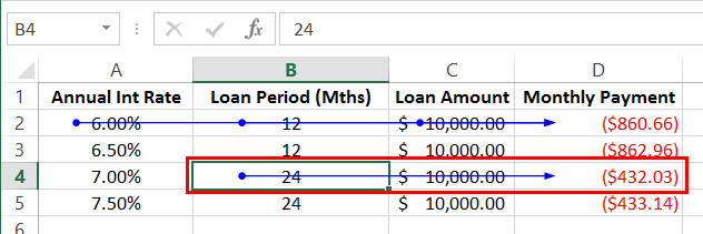
You will now see a blue arrow drawn across the current row, where all of the data used by the currently selected formula appears. Each blue dot on this arrow corresponds to a value that is used in the formula, while the arrowhead points to the end value. In this particular example, you can see that cells A2, B2, and C2 are all used by the formula in D2 to calculate the end value:

The Trace Dependents command works the opposite way of Trace Precedents: it highlights all the items that depend on the value in the current cell. This command will not work for values in the Monthly Payment column (D) because it has no dependents. However, the Loan Period (B) column does have dependents.
If we Click cell B4 and then click Formulas → Trace Dependents:

Another blue arrow will be drawn from the selected cell, pointing towards the dependent cell, which in this case is the formula in cell D4:

As you can see in the images, the Trace Precedents and Trace Dependents commands can be used at the same time.
To remove the arrows, click Formulas → Remove Arrows (drop-down arrow):

Clicking on the Formulas → Remove Arrows command directly will remove all arrows from the worksheet. The drop-down command allows you to remove all arrows, remove only precedent arrows, or remove only dependent arrows:

For this example, we have clicked Remove Arrows. All arrows on the current workbook will be removed:

Showing Formulas
When working with multiple formulas in your workbook, it is sometimes easier to view all of the formulas in the worksheet rather than their computed values.
To do this, click Formulas → Show Formulas:

All formulas will now be displayed in full. This command will also expand the column widths for all columns so that formulas are easier to read:

Click Formulas → Show Formulas again to return to the default view that shows calculated values and returns columns to their normal widths.
Evaluating Formulas
Tracing formula precedents and dependents allows you to quickly and accurately track what a selected formula is doing. The Evaluate Formula command takes this concept one step further by showing you every single calculation that was used by the formula to reach its end value.
To use this command, first select the cell that contains the formula that you would like to work with. For this example, we have selected cell D2:
Next, click Formulas → Evaluate Formula:

This action will open the Evaluate Formula dialog box, which will show the formula that will be evaluated. Click Evaluate to step into the first part of the formula:

In this case, you can see that “A2” in the formula was replaced to show “.06” (that cell’s actual value). Click the Step In button:
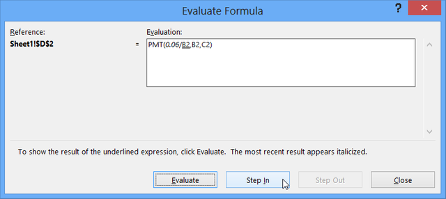
Clicking the Step In button will dive one level deeper in the formula, just as the Show Precedents/Show Dependents command would backtrack an additional level. Here, the value of B2 is shown in a separate text area. Click Step Out to hide the separate text area and progress to the next step:
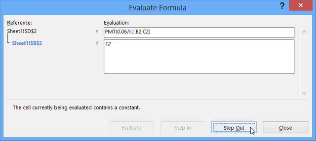
Now, the next value is highlighted and the option to step in is available again. Click Evaluate to continue:
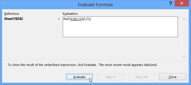
Continue clicking the Evaluate button to step through all the calculations one at a time. Stop when all the values of the formula are displayed and the entire formula is underlined. Click the Evaluate button once more:
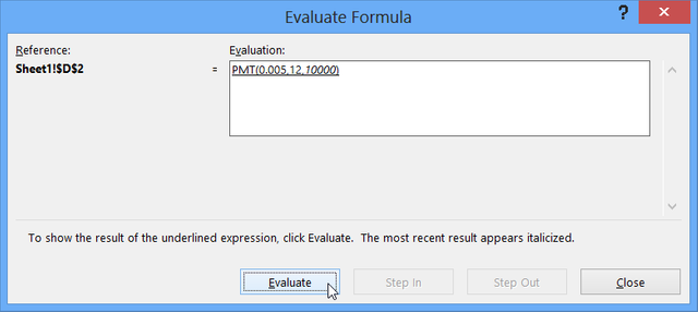
The end result of this formula will now be displayed:
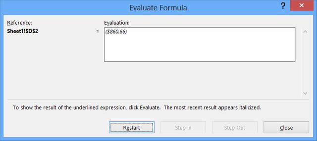
Clicking Restart will start the process over from the beginning. Click Close:

Setting Error Checking Options
Excel 2013 includes robust error checking features that have been refined over many different versions to catch just about any formula mistake. However, the effectiveness of error checking depends on Excel being properly configured.
To view and manage these settings, click File → Options:

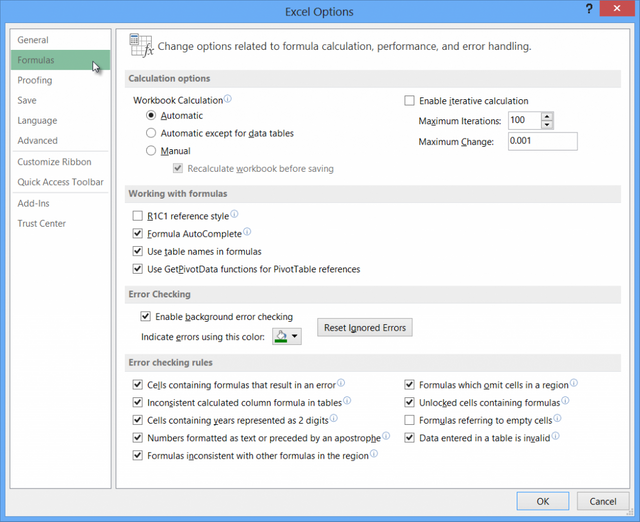
Then, click the Formulas category. Options to help you construct formulas and check them for errors can be found here:
Using Error Option Buttons
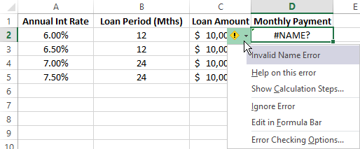
If automatic error checking is enabled, Excel will notify you when a formula error occurs. In the sample worksheet, cell D4 contains a #NAME? error. Click cell D4 and click the option button that appears:

If you hover over the option button, you will see a ScreenTip describing the error. Clicking the option button itself will show commands for resolving the error and modifying error checking options:
Click inside the worksheet to close the menu.
Running an Error Check
The Error Check feature works similar to the spell check feature found in most word processing applications. While Excel does actively check for errors while you are creating formulas, there are some problems that Excel’s automatic checking cannot account for.
Run an error check by clicking Formulas → Error Checking:

When the Error Checking tool is launched, it will immediately search your workbook for any formula errors. Any errors that are found will be listed one at a time. In this example, an error will be found in D2:
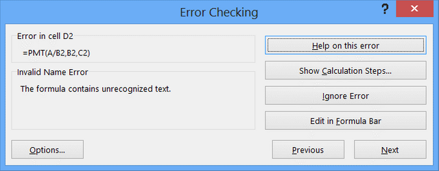
Cell D2 contains a naming error: the cell reference “A” is incomplete. You can use the buttons on the right to:
- Open the Help file for specific information about this error
- Show the calculation steps that were followed in order to reach this point
- Ignore this error for the time being
- Fix the error by hand with the formula bar
As well, the Options button will open the Excel Options dialog to the Formulas category, where you can customize Excel’s error handling settings.
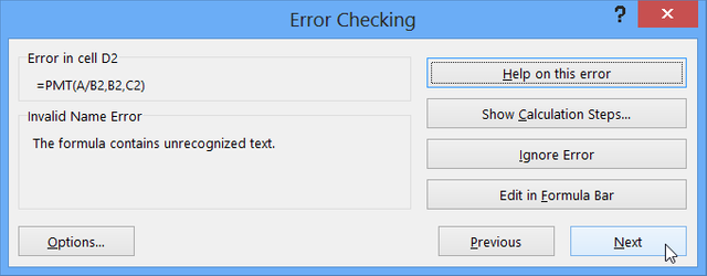
Click Next to move to the next error
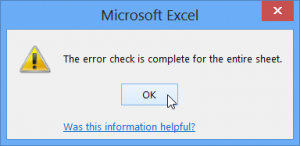
If no other errors are found in the current worksheet, a dialog will be displayed. Click OK:
Learn and Earn Activity
To earn STEEM tokens on this post, answer the following questions in the comments section below:
- Prior to reading this article, if you had an error on your spreadsheet, how did you resolve it?
- Now that you have a deeper understanding of the tools available in Excel to help with errors, what changes would you make in dealing with errors found on your spreadsheet?
Sign up to my newsletter for Excel and Power BI Tips, Ticks and Hacks
Sign Up Now
In return for this Tip – How to Resolve Errors in Excel Formula – I ask that you share this post or the video with your friends and colleagues

Now there is value in Learning with The Excel Club and our Learn and Earn STEEM activities.
We are the first Excel, PowerBI and DAX blog in the world where you can Earn while you Learn.
Find out more now and start earning while you are learning Excel and Power BI
Posted from my blog with SteemPress : http://theexcelclub.com/resolve-errors-in-excel-formula/
I never ran error checking on a full spreadsheet before, thanks for that. I did however resolve errors that were auto detected as they came up. its not something I would leave. Most of the time the errors were invalid so now I also know how to change the setting so they dont show up any more as errors. Thank you for this post Paula
Downvoting a post can decrease pending rewards and make it less visible. Common reasons:
Submit
Congratulations! Your post was discovered and featured by @OCD in its Reddit Compilation #3! The post was too old to receive a vote so we decided to vote on your most recent post :)
If you give @ocd a follow – you can find other Gems!
We also have a witness. You can vote for @ocd-witness with SteemConnect or on Steemit Witnesses to help support other undervalued authors!
Downvoting a post can decrease pending rewards and make it less visible. Common reasons:
Submit
Congratulations @theexcelclub! You have completed the following achievement on the Steem blockchain and have been rewarded with new badge(s) :
You can view your badges on your Steem Board and compare to others on the Steem Ranking
If you no longer want to receive notifications, reply to this comment with the word
STOPVote for @Steemitboard as a witness to get one more award and increased upvotes!
Downvoting a post can decrease pending rewards and make it less visible. Common reasons:
Submit