I released a backtesting engine in the article "Study on Multi-currency Hedging Strategy of Binance Futures" (https://www.fmz.com/digest-topic/5584). And the first report is based on the one hour K-line backtesting, which verifies the effectiveness of the strategy. However, as a matter of fact, the sleep time of the public strategy is 1s, which is a fairly high frequency strategy. It is obviously impossible to obtain accurate results by using the one hour K-line backtesting. Later, the results of "the minute-line backtest" was added (https://www.fmz.com/digest-topic/5621). As a result, the returns of backtesting has improved a lot, but it is still impossible to determine what parameters should be used in the second level case, and the understanding of the entire strategy is not very clear. The main reason is the important defects of backtesting based on the K-line.
Problems based on K-line backtesting
First of all, what is the historical K-line? One K-line data includes four prices: the highest price, opening price, the lowest price and closing price, starting time, end time and interval trading quantity. Most quantitative platforms and frameworks are backtested based on the K-line, and FMZ Quant Platform also provides Tick level backtesting. The speed of K-line backtesting is very fast, and it is no problem in most cases, but there are also very serious defects, especially the multi-variety strategy and high-frequency strategy of backtesting, which can hardly draw correct conclusions.
First of all, it is a matter of time. The time of the highest and lowest price of the K-line data is not given, so it is unnecessary to consider, but the most important opening and closing prices are not the opening and closing position times. Even if the trading varieties are unpopular, they are often not traded for more than ten seconds. When we backtest multiple-variety of strategies, we often default that their opening and closing prices are the same, which is also the basis of the closing price backtesting.
Imagine using the minute-line to backtest the arbitrage of two varieties. The difference between them is usually 10 yuan. Now it is found that at 10:01, the closing price of contract A is 100 yuan, the closing price of contract B is 112 yuan, and the difference is 12 yuan. So the strategy begins to hedge. At a certain time, the difference returns, and the strategy earns 2 yuan of return profits.
However, the actual situation may happen at 10:00:45, the contract A generated a transaction of 100 yuan, and then there was no transaction. Contract B generated a transaction of 112 yuan at 10:00:58. At 10:01, both prices did not exist. What was the opening price at this time? And how much difference could the hedging get? We don't know. One possible situation is that at 10:00:58, the trend of buying one and selling one of contract A is 101.9-102.1, and there is no spread of 2 yuan at all, which will mislead our strategy optimization greatly.
The second is matchmaking. The real matchmaking is price and time first. If the buyer exceeds the selling one price, he/she will generally conclude the transaction at the selling one price, otherwise, he/she will enter the order book and wait. It is obvious that the K-line data does not have the price of selling one or buying one, which is unable to simulate the matching at the level of detail.
The last is the impact of the transaction of the strategy itself on the market. If it is a small fund backtest, the impact will be small. However, if the trading quantity accounts for a large proportion, it will have an impact on the market. Not only will the price slip point be large when the transaction is completed immediately, but if your buying order is completed in the backtest, it actually preempts the transaction of other original traders who want to buy, which will have a butterfly effect impact on the market. However, this impact cannot be quantified, and it can only be said by experience that high-frequency trading can only accommodate small funds.
Backtesting based on real-time depth and tick
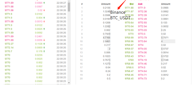
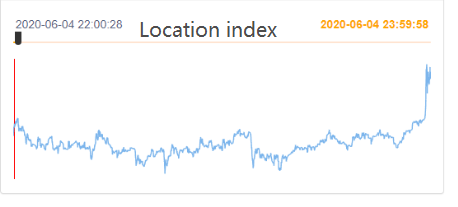
FMZ provides the real bot level backtesting, which can obtain the real historical 20-level depth, real-time second tick, transaction by transaction and other data, and based on this, it has made the real bot playback function (https://www.fmz.com/m/database). This kind of backtest measurement has a large amount of data and a slow speed, which can only be used for two days. For strategies that are relatively high frequency or require strict time judgment, the real bot backtesting is necessary. The trading pairs and time collected by FMZ are not too long, but there are more than 70 billion pieces of historical data. The current matching mechanism is that if the buying order is greater than the selling one order, it will be completely matched immediately without looking at the quantity, and if the buying order is less than the selling one order, it will enter the matching queue. This backtesting mechanism solves the first two problems of K-line backtesting, but it still cannot solve the last problem. And because the amount of data is too large, the backtest speed and time range are limited.


Backtesting mechanism based on transaction by transaction order flow
There is too little information about the K-Line, and the depth may also be false. However, one kind of data is the real transaction intention of the market, reflecting the most real transaction history - that is, transaction by transaction. In this paper, I will propose a high-frequency backtesting system based on the order flow, which will greatly reduce the amount of data in the backtesting at the real bot level, and to a certain extent, simulate the impact of trading volume on the market.
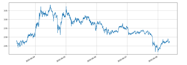
I downloaded the transaction by transaction of the last 5 days' Binance XTZ perpetual contract (download address: https://www.fmz.com/upload/asset/1ff487b007e1a848ead.csv). As a less popular variety, there are 213,000 pieces of data. Let's take a look at the composition of the data:
[['XTZ', 1590981301905, 2.905, 0.4, 'False\n'],
 ['XTZ', 1590981303044, 2.903, 3.6, 'True\n'],
 ['XTZ', 1590981303309, 2.903, 3.7, 'True\n'],
 ['XTZ', 1590981303738, 2.903, 238.1, 'True\n'],
 ['XTZ', 1590981303892, 2.904, 0.1, 'False\n'],
 ['XTZ', 1590981305250, 2.904, 0.1, 'False\n'],
 ['XTZ', 1590981305643, 2.903, 197.3, 'True\n'],
The data is a two-dimensional list, sorted by transaction time. The specific meanings are: species name, transaction price, transaction time stamp, transaction quantity, and whether the selling order is actively executed. There are both buying and selling. Each transaction includes the buyer and the seller. If the buyer is a market maker and the seller is an active transaction taker, the last data will be True.
First of all, according to the transaction direction, we can speculate the buy one and sell one in the market accurately. If it is an active selling order, the buy one price at this time is the transaction price. If it is an active buying order, the sell one price is the transaction price. If there is a new transaction, we will update the new opening position. If it is not updated, the last result will be retained. It is easy to launch the last moment of the above data. The buy one price is 2.903 and the sell one price is 2.904.
According to the order flow, it can be matched in this way: take a buying order as an example, the price is price, and the order quantity is amount. At this time, buy one and sell one of the opening position are bid and ask respectively. If the price is lower than ask and higher than bid, it will be judged as maker first, and priority can be given to matchmaking. Then all transactions with a transaction price lower than or equal to price during the order's lifetime will be matched with this order (if the price is lower than or equal to bid, priority cannot be given to the transaction, and orders with a transaction price lower than price will be matched with this order). The matchmaking price is price, and the transaction quantity is the transaction quantity of transaction by transaction, until the order is completely closed or cancelled. If the price is higher than ask, it will be judged as a taker. All subsequent transactions with a transaction price lower than or equal to price during the existence of the order will be matched with this order. The matching price is the transaction price of transaction by transaction. The distinction between maker and taker, because the exchanges encourage the pending orders with preferential service charges. For high-frequency strategies, this difference must be considered.
It is easy to see the problem of this matchmaking. If the order is a taker, the actual situation is that the transaction can be made immediately, rather than waiting for a new order to match it. First of all, we did not consider the number of orders listed on the market. Even if there were data, the direct judgment of the transaction has changed the depth and affected the market. The matchmaking based on new orders is equivalent to replacing your orders with the real orders in history, which will not exceed the transaction quantity limit of the market itself in any case, and the final profit cannot exceed the maximum profit generated by the market. Some of the matchmaking mechanism also affects the transaction quantity of orders, thereby affecting the returns of the strategy, which quantitatively reflects the strategy capacity. There will be no traditional backtesting, where the amount of returns doubled if the fund is doubled.
There are also some small details. If the buying price of an order is equal to the buy one price, there is still a certain probability that the order will be matched at the buy one price. The priority of the order and the transaction probability need to be considered, which is more complex, and it will not be considered here.
Matchmaking code
Exchange objects can refer to the introduction at the beginning, basically unchanged. Only the difference between maker and taker commissions is added, and the speed of backtesting is optimized. The matchmaking code is mainly introduced below.
    symbol = 'XTZ'
    loop_time = 0
    intervel = 1000 #The sleep time of the strategy is 1000ms
    init_price = data[0][2] #Initial price
    e = Exchange([symbol],initial_balance=1000000,maker_fee=maker_fee,taker_fee=taker_fee,log='') #Initialize the exchange
    depth = {'ask':data[0][2], 'bid':data[0][2]} #depth
    order = {'buy':{'price':0,'amount':0,'maker':False,'priority':False,'id':0},
             'sell':{'price':0,'amount':0,'maker':False,'priority':False,'id':0}} #Order
    for tick in data:
        price = int(tick[2]/tick_sizes[symbol])*tick_sizes[symbol] #Transaction price
        trade_amount = tick[3] #Number of transactions
        time_stamp = tick[1] #Transaction timestamp
        if tick[4] == 'False\n':
            depth['ask'] = price
        else:
            depth['bid'] = price

        if depth['bid'] < order['buy']['price']:
            order['buy']['priority'] = True
        if depth['ask'] > order['sell']['price']:
            order['sell']['priority'] = True
        if price > order['buy']['price']:
            order['buy']['maker'] = True
        if price < order['sell']['price']:
            order['sell']['maker'] = True

        #Order network delay can also be used as one of the matching conditions, which is not considered here
        cond1 = order['buy']['priority'] and order['buy']['price'] >= price and order['buy']['amount'] > 0
        cond2 = not order['buy']['priority'] and order['buy']['price'] > price and order['buy']['amount'] > 0
        cond3 = order['sell']['priority'] and order['sell']['price'] <= price and order['sell']['amount'] > 0
        cond4 = not order['sell']['priority'] and order['sell']['price'] < price and order['sell']['amount'] > 0

        if cond1 or cond2:
            buy_price = order['buy']['price'] if order['buy']['maker'] else price
            e.Buy(symbol, buy_price, min(order['buy']['amount'],trade_amount), order['buy']['id'], order['buy']['maker'])
            order['buy']['amount'] -= min(order['buy']['amount'],trade_amount)
            e.Update(time_stamp,[symbol],{symbol:price})
        if cond3 or cond4:
            sell_price = order['sell']['price'] if order['sell']['maker'] else price
            e.Sell(symbol, sell_price, min(order['sell']['amount'],trade_amount), order['sell']['id'], order['sell']['maker'])
            order['sell']['amount'] -= min(order['sell']['amount'],trade_amount)
            e.Update(time_stamp,[symbol],{symbol:price})

        if time_stamp - loop_time > intervel:
            order = get_order(e,depth,order) #Trading logic, not given here
            loop_time += int((time_stamp - loop_time)/intervel)*intervel
Some details should be noted:
- When there is a new transaction, we should match the order first, and then place the order according to the latest price.
- Each order has two attributes: maker -- whether it is maker, and priority -- matchmaking priority. Taking the buying order as an example, when the buying price is less than the selling one price, it is marked as maker, and when the buying price is greater than the buying one price, it is marked as priority matchmaking. Priority determines whether to match if the price equals the buying price, and maker determines the commission.
- The maker and priority of the order are updated. For example, there is a large purchase order that exceeds the opening positions, when there is a price greater than the buy price, at this time, the remaining transaction quantity will be maker.
- The intervel of the strategy is necessary, which can represent the delay of the market.
Backtesting of grid strategies
Finally, we reach the actual backtesting stage. Here, we are going to backtest a most classic grid strategy to see if it has achieved the expected effect. The strategy principle is that every time the price increases by 1%, we will hold a certain value of short position orders (otherwise, we will hold long position orders), and we will calculate the buy order and sell order and pend them in advance. The code will not be released. Encapsulate all codes into the function Grid ('XTZ ', 100,0.31000, maker_fee=-0.00002, taker_fee=0.0003). The parameters are: trading pair, holding value with price deviation of 1%, order density of 0.3%, sleep interval of ms, pending order comission, and taker comission.
XTZ market has been in shock in the last 5 days, which is very suitable for grid strategy.

We will backtest the impact of different positions on returns first. The returns measured by the traditional backtesting mechanism will certainly increase proportionally with the increase of positions.
e1 = Grid('XTZ',100,0.3,1000,maker_fee=-0.00002,taker_fee=0.0003)
print(e1.account['USDT'])
e2 = Grid('XTZ',1000,0.3,1000,maker_fee=-0.00002,taker_fee=0.0003)
print(e2.account['USDT'])
e3 = Grid('XTZ',10000,0.3,1000,maker_fee=-0.00002,taker_fee=0.0003)
print(e3.account['USDT'])
e4 = Grid('XTZ',100000,0.3,1000,maker_fee=-0.00002,taker_fee=0.0003)
print(e4.account['USDT'])
A total of four groups were backtested with position values of 100, 1000, 10000 and 100000, and the total backtesting time was 1.3s. The results are as follows:
{'realised_profit': 28.470993031132966, 'margin': 0.7982662957624465, 'unrealised_profit': 0.0104554474048441, 'total': 10000028.481448, 'leverage': 0.0, 'fee': -0.3430967859046398, 'maker_fee': -0.36980249726699727, 'taker_fee': 0.026705711362357405}
{'realised_profit': 275.63148945320177, 'margin': 14.346335829979132, 'unrealised_profit': 4.4382117331794045e-14, 'total': 10000275.631489, 'leverage': 0.0, 'fee': -3.3102045933457784, 'maker_fee': -3.5800688964477048, 'taker_fee': 0.2698643031019274}
{'realised_profit': 2693.8701498889504, 'margin': 67.70120400534114, 'unrealised_profit': 0.5735269329348516, 'total': 10002694.443677, 'leverage': 0.0001, 'fee': -33.984021415250744, 'maker_fee': -34.879233866850974, 'taker_fee': 0.8952124516001403}
{'realised_profit': 22610.231198585603, 'margin': 983.3853688758861, 'unrealised_profit': -20.529965947304365, 'total': 10022589.701233, 'leverage': 0.002, 'fee': -200.87094000385412, 'maker_fee': -261.5849078470078, 'taker_fee': 60.71396784315319}
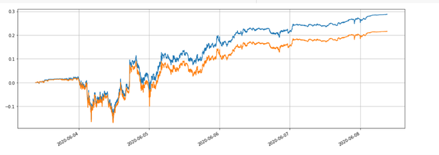
It can be seen that the final realized profits are 28.4%, 27.5%, 26.9% and 22.6% of the position value respectively. This is also in line with the actual situation. The greater the value of the position is, the greater the value of the order will be, and the more likely partial transactions will occur. The final realized returns will be smaller relative to the amount of the order. The figure below shows the comparison of relative returns with position values of 100 and 10000 respectively:

We can also backtest the impact of different parameters on the return of the backtest, such as the pending order density, sleeping time and commissions. Take the sleep time as an example, change it to 100ms, compare with the sleep time of 1000ms, and observe the returns. The backtesting results are as follows:
{'realised_profit': 29.079440803790423, 'margin': 0.7982662957624695, 'unrealised_profit': 0.0104554474048441, 'total': 10000029.089896, 'leverage': 0.0, 'fee': -0.3703702128662524, 'maker_fee': -0.37938946377435134, 'taker_fee': 0.009019250908098965}
The profit has increased a little. This is because only one group of orders are pending to the strategy, and some orders cannot get the fluctuating price because they have no time to change. The reduced sleep time improves this problem. This also shows the importance of pending multi-group orders in grid strategy.
Summary
This paper proposes a new backtesting system based on the order flow innovatively, which can partly simulate the matching situation such as order pending, order taking, partial transaction and delay, partly reflects the impact of strategic fund volume on returns, and it has important reference value for high-frequency strategies and hedging strategies. High precision backtesting points out the direction for the optimization of strategy parameters. It has also been verified by long-term real bot tests. And the amount of data required for backtest is well controlled, and the backtest speed is also very fast.